If you’ve just started learning how to use Microsoft Excel, you’ll probably have a lot of questions to ask about the functions of the program. Because let’s face it, despite being exceptionally useful, Excel can be a very complicated application. It’s like a hammer when your most frustrating reporting tasks at work resemble nails.
Aside from great Excel features such as flash fill, pivot tables, and conditional formatting, Excel also has a lot of powerful functions that will help save time when creating spreadsheets. Invest some time in learning to use Excel so you can prepare and manage complex reports, as well as perform what-if analysis on data like a pro!
To help you get started, here are 5 important Excel functions you should learn today.
1. The SUM Function
The sum function is the most used function when it comes to computing data on Excel. This function works to sum a group of numbers in a specific set of cells. This means you don’t need to type a long cumbrous formula just to calculate the sum of all the data you need. Because of its popularity, newer versions of Microsoft Excel have a button specifically for this function.
This function is performed by typing the formula on the function bar and highlighting the cells you want summed before clicking “Enter”. You also need to be careful in highlighting cells, as Excel will sum everything you include. If this happens, you can easily click the “Undo” button to reset the values back to its original state.
The syntax formula for sum function is “=SUM” (number1, number2, etc.).
In this image, the sum function for the cells C2 through C7 is obtained through the formula “=SUM(C2:C7)”, giving you the result of 33161.
2. The TEXT Function
Text function is a useful tool that helps convert a date (or number) into a text string in a particular format. It falls in the category of string formulas that converts numerical values to a string. It is handy when users need to view numeric data in a readable format. Take note that the “TEXT” formula only works to convert numeric values to text. Therefore, its results cannot be calculated.
The syntax formula for text function is “=TEXT” (value, format_text).
- “Value” refers to the particular number you wish to convert to text.
- “Format_text” defines the format of the conversion.
In this example, the user uses a text formula to find the abbreviated day for the date “=TEXT (B2, “ddd”)”.
3. The VLOOKUP Function
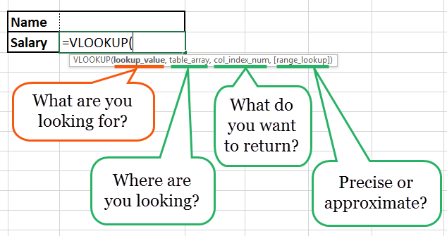
VLookup is powerful Excel function that is often overlooked. Users will find it useful when they need to find specific data on a large table. You can also use VLookup to search for names, phone number, or specific data on your sheet. Instead of manually looking for the names and wasting time scrolling through hundreds of data, the VLookup function makes this process faster and more efficient.
Image: spreadsheeto.com
The VLookup formula is “=VLOOKUP” (lookup_value, table_array, col_index_num, *range_lookup*).
- “lookup_value” is the data you want to find.
- “table_array” is the data column where you want to limit your search.
- “col_index_num” is the column number within the table that you want to return a value from.
- “range_lookup” is an optional argument that allows you to search for the exact match of your lookup value without sorting the table.
4. The AVERAGE Function
The average function is an extremely useful tool for getting the average value in a range of cells. Like the sum function, it is frequently used in computing and analyzing data on spreadsheet. Basically, the average function works to find the “arithmetic mean” for a group of cells. Aside from the average function, Excel also has the median and mode function.
The syntax formula for the average function is “AVERAGE” (number1, number2, etc.).
- “Number 1” refers to the first number in the range where you want the average.
- “Number 2” is the additional reference of the average range. You can get an average of up to a maximum of 255 cells.
Additional Examples:
“=AVERAGE (A2:A10)” – computes the average of numbers in cells A2 through A10.
“=AVERAGE (B2: B10, 7)” – computes the average of the numbers in cells B2 through B10 and the number 7.
5. The CONCATENATE Function
This function is a good time saver when you need to combine data from 2 or more cells. Unlike the merge tool which physically merges two or more cells into a single cell, the concatenate function only combines the contents of the combined cells. In the latest version of Excel ( 2016), the concatenate function has been replaced with concat function and will be incorporated in more future versions of Excel.
The syntax formula for the concatenate function is “CONCATENATE” (text1, [text2…text_n]),
- “Text1, Text2…text_n” are the data you want to combine.


